Project
Neural Network Quantization
keywords: squeezeNet, resNet 18/34/50, model quantizaton, post traning quantization, pytorch
date: Sep.2021
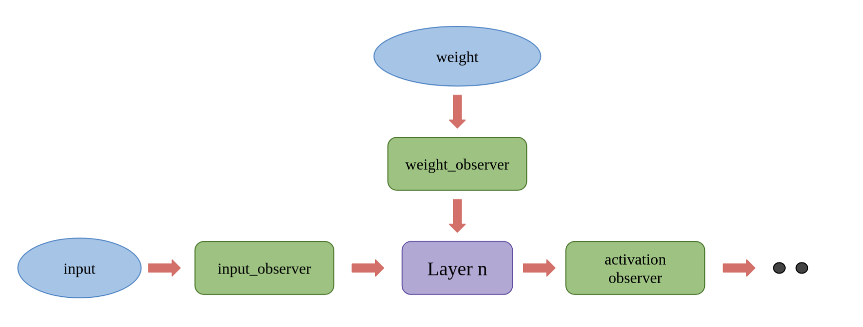
Nowadays in deep learning field, using parameters with 32-bit floating point format is the mainstream, also Known as FP32. Despite the higher accuracy from the FP32 format, the training is computationally expensive. Model Quantization will significantly reduce the bandwidth and storage of the neural network, which brings the possibility of implementing the model on those devices without GPU. Research has proved that weights and activations can be represented using 8-bit integers (or INT8) without incurring significant loss in accuracy. The principal idea of Parameter quantization is to train a quantizer that learns a mapping function between input and output, so that such function will convert a larger set of input values into a smaller set of output value. Currently both newest Pytorch (1.9.0) and tensorflow (2.4.0) can provide user-friendly model quantization functions.
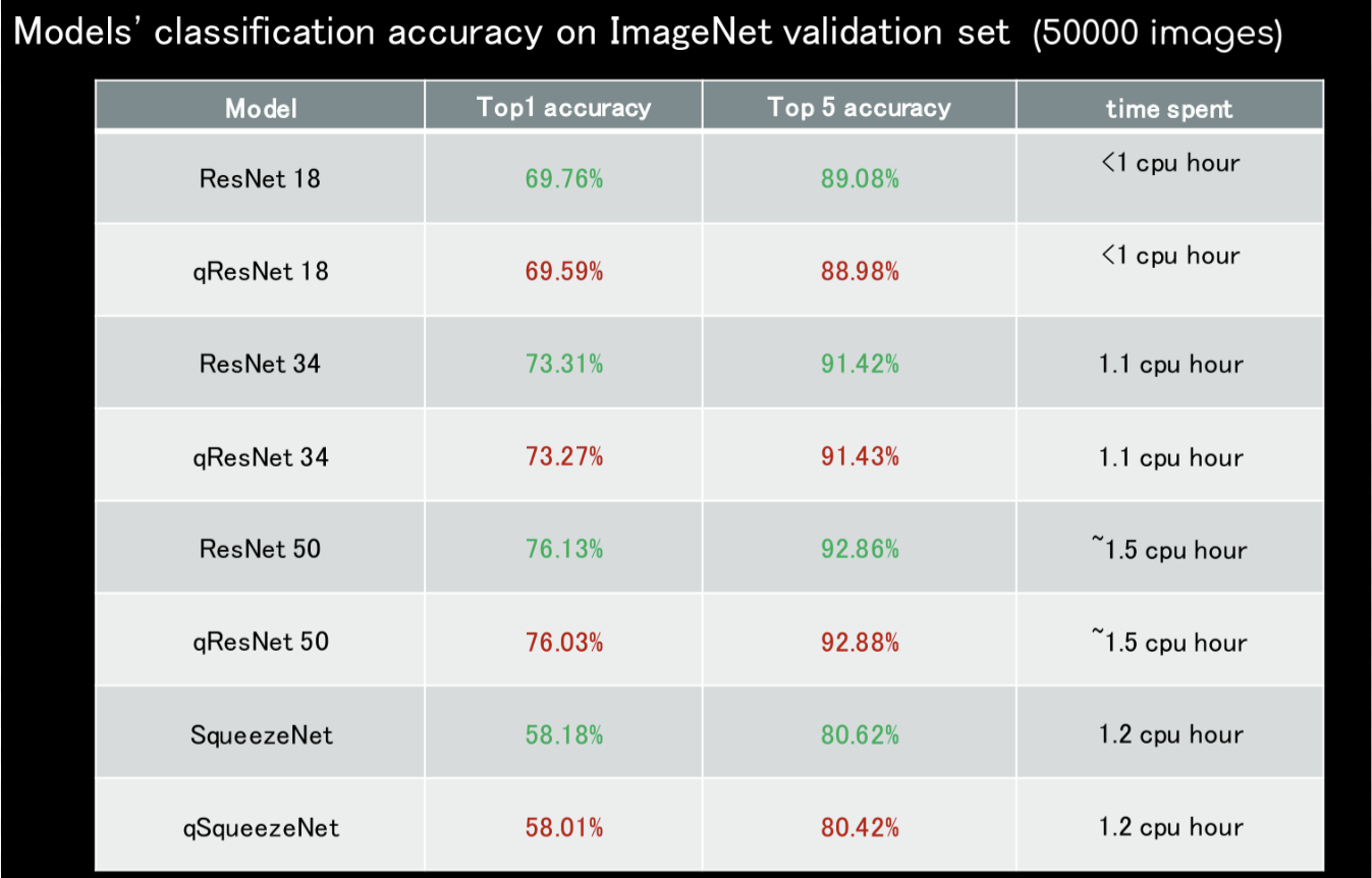
Considering that so far all the quantization frameworks are beta version. We build a model quantization library base on pytorch (1.9.0), which provide us more flexibilities in observer selection, model fusing and quantization hyperparameter searching. Importantly, our quantized models have better performance than other resources. We conduct post traning quantization experiments on SqueezeNet, ResNet18/34/50; then check the qModels' classification accuracy on ImageNet validation set. The results are shown in the below figure. By using int8 parameters, we lost less than 0.25% accuray. Super cool work, isn't it?
SSD-ResNet50 INT8 Quantization
keywords: SSD, resNet50, object detection, neural network quantization, pytorch, coco2017
date: November.2021
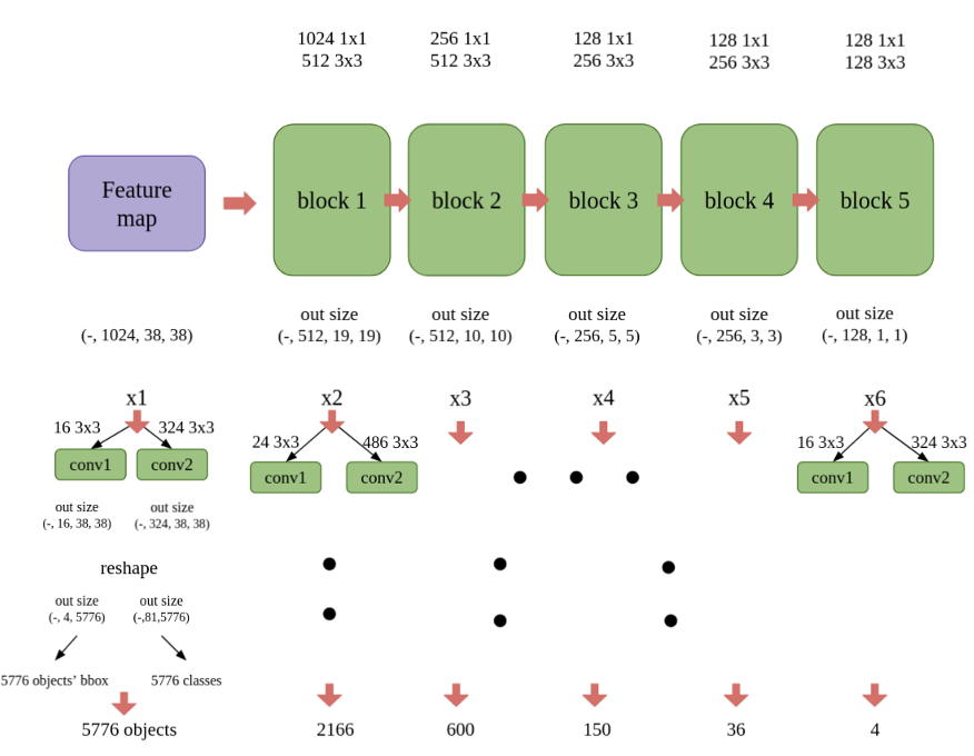
Single Shot MultiBox Detector (SSD) is a one-stage object detector that predicts bounding boxes and class scores directly from a set of feature maps, without a separate region-proposal network. In this project we study an SSD300 with a ResNet50 backbone, evaluate its detection accuracy on COCO2017, and then push it through post-training quantization in PyTorch to see how far we can compress it while keeping the mAP intact.
The pipeline has three main stages:
- Run the backbone (ResNet50) to produce a feature map of shape (batch, 1024, 38, 38).
- Extract a multi-scale feature pyramid [x1, x2, x3, x4, x5, x6] through 6 detection blocks (1x1 conv followed by 3x3 conv).
- For every pixel of every level, regress [4, 6, 6, 6, 4, 4] default boxes and classify them, yielding 8732 candidate objects; the final predictions are obtained by per-class non-max suppression.
SSD outputs two tensors per image: loc with shape [batch, 4, 8732] and conf with shape [batch, 81, 8732] (80 COCO classes + background). For each class we keep boxes with confidence > 0.05, sort them, and iteratively suppress the ones whose IoU with an already-kept box exceeds 0.5.
Evaluating detection accuracy
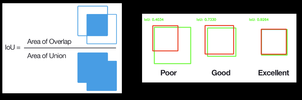
To measure the model we use the COCO metric mean Average Precision at IoU = 0.5:0.05:0.95. The Intersection over Union (IoU) between a prediction and the ground truth tells us whether the box should be counted as a true positive (IoU ≥ 0.5), a false positive (IoU < 0.5 or duplicated box), or a false negative (a missed ground-truth object). True negatives are not used, since the background covers most of the image.
By sweeping the IoU threshold from 0.5 to 0.95 (step 0.05) and averaging the per-class APs, we get the standard COCO mAP. We further break the score down by object area (small / medium / large) and by the maximum number of detections kept per image (maxDets = 1, 10, 100), which is useful to spot whether the model loses small objects after quantization.
Quantization plan and findings
Starting from a pretrained float SSD with mAP = 0.253 on COCO2017 val, we run post-training quantization in two steps: first quantize only the backbone ("half-quantized SSD") and then the whole detector. This isolates the contribution of each part to the accuracy drop.
- Calibration data matters. A naive run with the NVIDIA training loader (which produces tensors in [0, 1]) and the validation loader (ImageNet-normalized to roughly [-2.12, 2.64]) collapsed the half-quantized model to 0.107 mAP. Re-calibrating with 20 batches taken directly from the validation set, whose statistics match the inference pipeline ([-1, 1]), recovers 0.2503 mAP — only 0.003 below the float baseline.
- Histogram > MinMax. Because the backbone produces a long-tailed activation distribution (SSD layer3 max ~17.1 vs ~3.35 for plain ResNet50), the MinMax observer wastes resolution on outliers. Switching to a full Histogram observer drops the layer-3 L1 quantization error from 0.0328 to 0.0159; a percentile-clipped variant (97.5%, 99%, 99.5%, 99.7%) was actually worse than MinMax.
- Where the error lives. Layer-by-layer L1 analysis on the fully-quantized SSD shows that most of the quantization error is concentrated in the deeper backbone blocks and the first detection block, while the head convolutions stay benign — this matches the heavy, wide activation distributions seen in those layers.
The take-away is that for one-stage detectors the bottleneck is not the detection head but the backbone activations, and the easiest 80% of the accuracy gap can be closed by (1) calibrating with samples drawn through the real inference pre-processing and (2) using a Histogram (or KL) observer instead of MinMax.
ResNet Quantization: Observers & Data Formats
keywords: ResNet18, ResNet34, ResNet50, post-training quantization, FuseConvAdd, histogram observer, pytorch, ImageNet
date: Sep.2021
This is a focused study of post-training quantization on the ResNet family (18 / 34 / 50) in PyTorch. Starting from torchvision pretrained weights, we calibrate each network with a small slice of the ImageNet training set (10–20 batches, ~800 images) and evaluate the int8 model on the full 50,000-image ImageNet validation set. The 10-run experiments report (max / min / mean) to capture run-to-run variance from random calibration sampling.
Three design choices were studied independently to understand where the quantization error is born and how to close the gap with float32:
- Residual connection. A vanilla QAdd layer vs a fused QFuseConvAdd layer that absorbs the conv into the add. For the basic block with a downsample shortcut (figure below), QFuseConvAdd has two flavours: fuse the conv path first then add the residual, or fuse the residual path first then add the conv — the first one has the smaller layer-wise L1 error.
- Final FC layer. With vs without an explicit re-quantization step (doRequantize) on its input.
- Activation observer. MinMax vs Histogram.
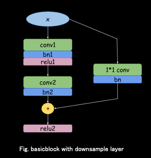
Basic block with a 1×1 downsample shortcut — the residual path that QFuseConvAdd targets.
Master comparison table
All numbers below are Top-1 / Top-5 accuracy on the full ImageNet validation set (50k images). For 10-run experiments the mean is shown; one-shot experiments are marked with †. Δ is the Top-1 gap to the corresponding float32 baseline. The final recipe for each network is highlighted.
| Model | Residual | FC doReq | Observer | DType | Top-1 | Top-5 | L1 err | ΔTop-1 |
|---|---|---|---|---|---|---|---|---|
| ResNet 18 | — | — | — | FP32 (fused) | 69.76 | 89.08 | — | — |
| qResNet 18 | QAdd | yes | MinMax | int8 | 69.51 | 88.94 | — | −0.25 |
| qResNet 18 | QFuseConvAdd | no | MinMax | int8 | 69.56 | 88.96 | — | −0.20 |
| qResNet 18 | QFuseConvAdd | no | Histogram | int8 | 69.59† | 88.98 | 0.1084 | −0.17 |
| qResNet 18 | QFuseConvAdd | no | Histogram | FP16 | 69.53 | 89.01 | — | −0.23 |
| qResNet 18 | QFuseConvAdd | no | Histogram | BF16 | 69.56 | 88.96 | — | −0.20 |
| ResNet 34 | — | — | — | FP32 (fused) | 73.30 | 91.42 | — | — |
| qResNet 34 | QAdd | yes | MinMax | int8 | 73.18 | 91.36 | — | −0.12 |
| qResNet 34 | QFuseConvAdd | yes | MinMax | int8 | 73.16 | 91.41 | — | −0.14 |
| qResNet 34 | QFuseConvAdd | no | MinMax | int8 | 73.21† | 91.42 | 0.1395 | −0.09 |
| qResNet 34 | QFuseConvAdd | no | Histogram | int8 | 73.27† | 91.43 | 0.1023 | −0.03 |
| qResNet 34 | QFuseConvAdd | no | Histogram | FP16 | 73.24 | 91.40 | — | −0.06 |
| qResNet 34 | QFuseConvAdd | no | Histogram | BF16 | 73.18 | 91.34 | — | −0.12 |
| ResNet 50 | — | — | — | FP32 (fused) | 76.15 | 92.87 | — | — |
| qResNet 50 | QFuseConvAdd | yes | MinMax | int8 | 75.81 | 92.81 | — | −0.34 |
| qResNet 50 | QFuseConvAdd | no | MinMax | int8 | 75.89† | 92.84 | 0.1876 | −0.26 |
| qResNet 50 | QFuseConvAdd | no | Histogram | int8 | 76.03† | 92.88 | 0.1359 | −0.12 |
| qResNet 50 | QFuseConvAdd | no | Histogram | FP16 | 75.92 | 92.89 | — | −0.23 |
| qResNet 50 | QFuseConvAdd | no | Histogram | BF16 | 75.83 | 92.85 | — | −0.32 |
Highlighted rows: final recipe per network. †single run; all other int8 rows are the mean of 10 runs.
Take-aways
- With the right recipe, int8 ResNet 18/34/50 lose only 0.03–0.17% Top-1 versus float32 on ImageNet, well within run-to-run noise.
- Histogram beats MinMax by ~0.1–0.15 Top-1 on ResNet 50 and reduces the FC-input L1 error by ~25%.
- Fuse addition and conv operations on the residual branch and an FC layer without a leading re-quantization improves both accuracy and inference-time performance.
- Going from FP32 to FP16 on the DPU is essentially lossless; BF16 costs about 0.2% Top-1 and may be acceptable depending on the deployment budget.
YOLOv3–v5 INT8 PTQ
keywords: YOLOv3, YOLOv4, YOLOv5, object detection, post-training quantization, int8, pytorch, coco2017
date: June.2022
The YOLO family is the most successful one-stage object detectors deployed in industry: it consistently lands the best accuracy / FPS trade-off on COCO, and the open ecosystem (Ultralytics + many forks) makes it the de-facto starting point for real-time vision pipelines on edge devices. In this project I take YOLOv3, YOLOv4 (incl. CSPx) and the full YOLOv5 family (n / s / m / l, plus ReLU variants) and quantize them to int8 with post-training quantization only — no fine-tuning. With a handful of model-specific tricks (I invented), all networks land within ~1% mAP of float, and the most accurate ones (YOLOv4-CSPx, YOLOv5s-ReLU) within ~0.2–0.7%, which is state-of-the-art for PTQ.
YOLOv5 architecture overview
YOLOv5 keeps the three-stage design that has defined the family since v3: a CSP-style BackBone for feature extraction, a PANet-based neck that fuses features at three resolutions (top-down + bottom-up), and three Conv1×1 detection heads predicting class scores and bounding boxes per anchor. The basic block evolves at every version: v3 uses a Conv-BN-LeakyReLU residual unit, v4 introduces a CSP split with Mish, and v5 keeps the CSP topology with the smoother SiLU activation.
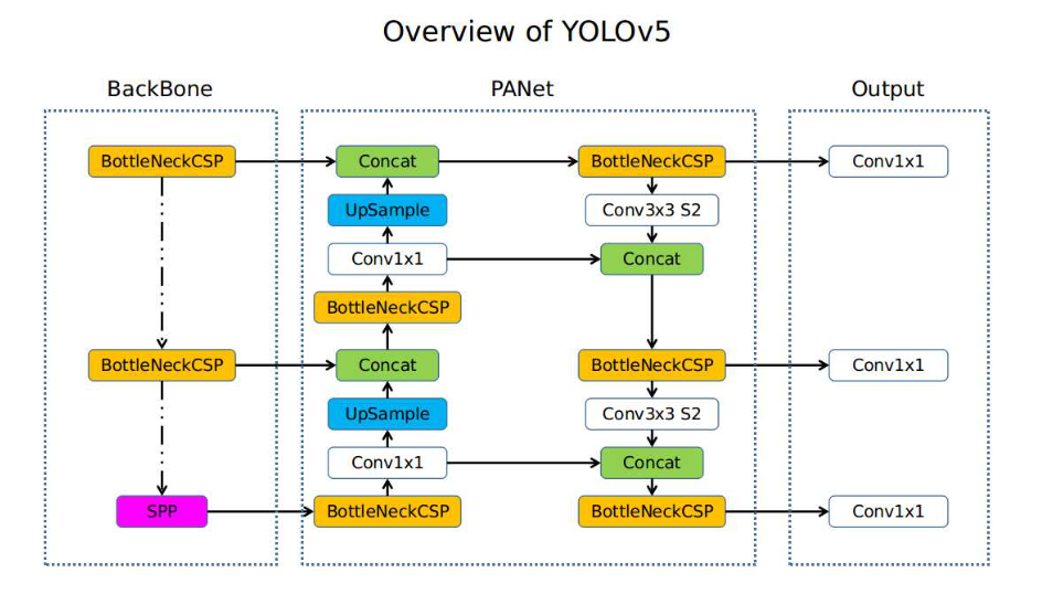
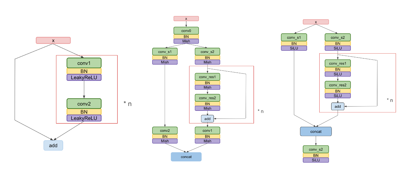
Left: full YOLOv5 graph (BackBone → PANet → 3 detection heads). Right: basic block evolution — v3 (LeakyReLU), v4 (CSP + Mish), v5 (CSP + SiLU).
PTQ results on COCO 2017 val (mAP @ 0.5:0.95)
All quantized models are evaluated on the COCO 2017 validation set at 640×640 input. Official is the number reported by the original repo, ModelZoo is our reproduced float32 baseline, and INT8 (PTQ) is the post-training-quantized version using the tricks mentioned above. Diff is the mAP gap between INT8 and the ModelZoo float baseline.
| Model | Official | ModelZoo (640×640) | INT8 (PTQ) | Diff |
|---|---|---|---|---|
| YOLOv3 | — | 39.86% | 39.03% | 0.83% |
| YOLOv4 | — | 50.73% | 49.97% | 0.76% |
| YOLOv4-CSPx | — | 52.94% | 52.73% | 0.21% |
| YOLOv5n | 28.0% | 28.1% | 27.3% | 0.8% |
| YOLOv5s | 37.4% | 37.4% | 36.55% | 0.85% |
| YOLOv5m | 45.4% | 45.3% | 44.25% | 1.05% |
| YOLOv5l | 49.0% | 49.0% | 47.47% | 1.53% |
| YOLOv5s-ReLU | 34.2% | 35.4% | 34.72% | 0.68% |
| YOLOv5m-ReLU | 43.5% | 43.5% | 42.7% | 0.8% |
Best PTQ gap per family in bold. Highlighted rows: SiLU→ReLU and CSPx variants where careful block fusion shrinks the gap most.
Take-aways
- All YOLO networks PTQ-quantize to within roughly 0.2–1.5% mAP of their float32 baseline, with no fine-tuning required.
- Activation function matters even more: replacing SiLU with ReLU (YOLOv5s-ReLU, YOLOv5m-ReLU) shrinks the int8 gap meaningfully — ReLU is more friendly to our hardware.
- Requires to implement many tricks to achieve good PTQ accuracy.
INT8 Multi-Object Tracking
keywords: ByteTrack, multi-object tracking, Kalman filter, post-training quantization, int8, MOT17
date: June.2023
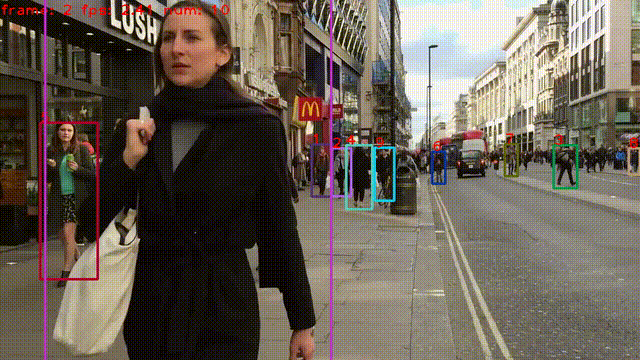
ByteTrack is a strong tracking-by-detection method for multi-object tracking, built around a YOLOX-style detector. Its core idea is simple but highly effective: rather than discarding low-confidence detections, ByteTrack performs a second association stage to match them with tracks that remain unmatched after the first pass. Together with a per-track Kalman filter for motion prediction and IoU-based data association, this helps recover trajectories that conventional SORT-style trackers often fragment or lose.
ByteTrack series achieves state-of-the-art MOTA on MOT17 and MOT20 while maintaining real-time performance. The demo below shows a quantized ByteTrack model running on CUDA on a 720p video sequence.
Where does the per-frame time actually go?
ByteTrack's tracking step has two main CPU-side costs: (i) the first-step Kalman filter that predicts the next box for every active track, and (ii) the IoU matching that pairs predicted tracks with new detections via the Hungarian algorithm. We profiled both as a function of the number of active tracks on a 720p stream:
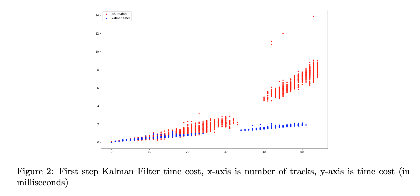
Per-frame time cost vs. number of active tracks. Blue: Kalman filter prediction. Red: IoU matching.
Two observations come out of the plot:
- The Kalman filter stays essentially flat at ~1–2 ms per frame, even when the scene contains 50+ tracks. Vectorising the predict step over all tracks at once is enough to keep it bounded.
- The IoU matching grows roughly linearly-to-quadratically with track count and becomes the dominant cost above ~30 tracks (6–14 ms per frame on busy frames). So if you want to speed up ByteTrack on crowded scenes, the matching step — not the Kalman filter — is where to spend the optimization budget.
PTQ results on a 720p video
I managed to quantized all the ByteTrack versions (detecor) to int8 with post-training quantization only and ran the full tracker on a 720p video. Accuracy is reported as MOTA (%); Official is the number from the ByteTrack repo. Due to the hardware setting, I used fixed input size 640×640.
| Model | Official | My implementation (640×640) | INT8 (PTQ) | Diff |
|---|---|---|---|---|
| ByteTrack-n | 69.0% | 70.3% | 70.0% | 0.3% |
| ByteTrack-t | 77.1% | 76.5% | 76.6% :) | 0.1% |
| ByteTrack-s | 79.2% | 79.7% | 79.4% | 0.3% |
| ByteTrack-m | 87.0% | 87.2% | 87.0% | 0.2% |
ByteTrack-t is the happy outlier: the int8 model is actually 0.1% better than its float32 baseline.
Take-aways
- All four ByteTrack variants quantize to within 0.1–0.3% MOTA of float32, with no fine-tuning needed.
- The Kalman filter prediction is not the tracker's bottleneck — the IoU matching step dominates as track count grows, so int8 quantization of the detector buys real end-to-end FPS gains.